Generators
Modifiers
constant
list
segment function
random generator
probability generator
oscillator
Every event or note in a Csound score is described by an i statement and controlled by a number of
parameters, called pfields p1,p2,p3 ... These pfields contain
instrument number, onset time (or beat) and duration of each event.
Moreover it is possible to define other parameters for the
instruments numbered as p4,p5 etc. These are usually
frequencies or pitches, transpositions, filter values, amplitudes,
attack times, panorama positions, table numbers and so on.
One parameter in CMask corresponds to
one pfield of an i statement in Csound. The first parameter is the
instrument number p1. The
second parameter, in Csound actually the onset time (or the beat,)
will be regarded as the onset difference (or the rhythm) between
successive events. The sum of all preceeding onset differences up to
a certain event gives us the absolute onset time p2 of this event. The p2 parameter in CMask has another special
quality: it determines the event density, that is how many notes will
be generated in a certain time span. The third is the duration
p3. Every subsequent
parameter gets its meaning from the orchestra file.
The instructions for the parameter generation take place in a special text file called the parameter file .
Normally all the events or grains have the same or similar
properties so they can be grouped together from a statistical point
of view. These groups or rather the parameters of their events called
fields in CMask. The notion of fields is
comparable to clouds or streams in other concepts of granular
synthesis. A field has a duration that is determined by start and end
time. The values of each paramter p1,p2,p3 ... pn within this time span can be
generated and processed by different means. At first, one of the
generators (see below) produces a value.
This might be a random or a periodical value or one from a list of
fixed numbers. The value can be now processed or modified with up to
3 modules (tendency mask, quantizer,
accumulator) in dependence on the generator type. (For example: a
list can't be followed by a mask but by an accumulator.)
With the mask module the generated values will be mapped into a time variant domain - the tendency mask. The quantizer adjusts its input values (the values from a mask or a generator) to a time variant grid. The last module, the accumulator, sums all values together. These 3 modifiers are optional.
|
Generators |
Modifiers | |||||
|---|---|---|---|---|---|---|
|
| ||||||
|
constant |
|
|
|
|
|
|
|
list |
|
|
|
|
|
|
|
segment function |
|
|
|
|
|
|
|
random generator |
|
|
|
|
|
|
|
probability generator |
|
|
|
|
|
|
|
oscillator |
|
|
|
|
|
|
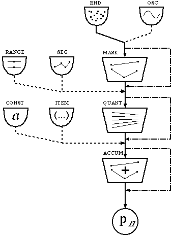
Most of the modules can be controlled by special parameters. These control parameters can be constant or time dependent. The variable parameters will be described by segment functions:
Segment functions (or break point functions) serves in CMask both as generators of event parameters and as control functions for special generator and modifier parameters. Such special parameters are, for example, the mean value of a gaussian probability distribution, the quantization strength or a boundary of a tendency mask.
A segment functions consists, like the linseg and expseg unit generators and GEN5 / GEN7 in Csound, of a connected sequence
of segments. The segments are determined by pairs of time and related
function values.
Values between these points will be calculated by an interpolation. There is a linear, a power or a
half-cosine function interpolation. The interpolation type is set by
an exponent (see below and in the reference section). It can also be
set off - the result is a
step function similar to Csounds GEN17.
(0 0 4 10 7 5 9 8 ipl 0.5)
resp. (0 0 4 10 7 5 9 8
ipl 2)
(0 0 4 10 7 5 9 8 ipl -0.5)
resp. (0 0 4 10 7 5 9 8
ipl -2)

(0 0 4 10 7 5 9 8 ipl
   0)

(0 0 4 10 7 5 9 8 ipl
   cos)
(0 0 4 10 7 5 9 8 ipl
   off)

The value of the first defined time-value pair of a segment function is also valid before this time (without interpolation). The same applies to the last defined value:

CMask generates random numbers either by a simple random generator (range) or by means of dynamic
controllable probability functions
(rnd).
The implemented probability distributions are: uniform, linear, triangle, exponential, bilateral and reverse exponential, gaussian, cauchy, beta and weibull. For a detailed description of these probabilities see in [a], [1], [2], [3].
Many of these distributions are controllable by one or two parameters. They can be set as constant or as variable by a segment function. A gaussian distribution, for example, is determined by a mean value and a standard deviation. If we vary the standard deviation the shape of the distribution (the histogramm) will be changed.
If we have the segment function pairs 0 1 and 10 3 as control values for an exponential distribution, the result is a rising exponent (lambda) from 1.0 at 0 seconds to 3.0 at 10 seconds, that is, the generator prefers more lower values at time 10.0.
If we have a cauchy distribution and control its mean value by 0 0.5 and 10 0.8, we get a mean value that changes from 50% to 80% of the range {0...1}.
The parameters for every probability function and their ranges are described in the reference section of this manual.
The generated random numbers are limited to the range {0...1} (even if they might be lower or higher in theory, like gaussian, cauchy, exponential and weibull). This range can be stretched or compressed by a subsequent tendency mask.
rnd uni

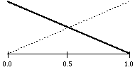
linear distribution
rnd lin 1
resp. rnd lin
-1
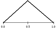
triangle distribution
rnd tri
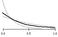
exponential distribution
rnd exp 1
resp. rnd exp 0.7
resp. rnd exp 2
reverse exponential distribution
rnd rexp 1
resp. rnd rexp 0.7
resp. rnd rexp 2
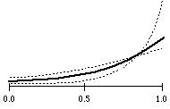
bilateral exponential distribution
rnd bexp 1
resp. rnd bexp 0.7
resp. rnd bexp 2
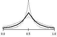
gaussian distribution
rnd gauss .5 .2
resp. rnd gauss .5 .1
resp. rnd gauss .2 .2
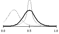
cauchy distribution
rnd cauchy .5 .2
resp. rnd cauchy .5 .15
resp. rnd cauchy .2 .2

beta distribution
rnd beta .2 .2
resp. rnd beta .6 .6
resp. rnd beta .1 .3
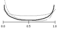
weibull distribution
rnd wei .5 3
resp. rnd wei .5 1
resp. rnd wei .5 .3

There are not only random generators in CMask. It is also possible to use the following periodic functions as parameter generators: sine, cosine, saw tooth up and down, square, triangle and periodic power functions.
Every function has a frequency value measured in cps, constant or time variant, and a constant phase (normalized, between 0 and 1). These functions produce values in the range {0...1}, like the random generators, i.e. their amplitudes keep constant.
A subsequent mask can serve as an amplifier to achieve other ranges.
sine function
osc sin 1

cosine function
osc cos 1

saw up function
osc sawup 1

saw down function
osc sawdown 1

power up function
osc powup 1 0 1
resp. osc powup 1 0 2
resp. osc powup 1 0
-1

power down function
osc powdown 1 0 1
resp. osc powdown 1 0 2
resp. osc powdown 1 0
-1

square function
osc square 1

triangle function
osc triangle 1

Instead of random or oscillating generators one can use simple lists.
A list contains a set of numbers, for example (5 1 8 10.2) or (1.5 0.01 0.01 1234) etc.
The elements of the list can be selected by different methods: in
a forward loop (cycle), in a forward and backward loop, like a pendulum or
a palindrome (swing), as
random permutations, like a stack of
cards (heap) and by chance (random). There is in contrast to
segment functions no time dependence at all - the elements will be
read one by one corresponding to the mode.
The example shows the four modes with the same list:
item cycle (1 2 3 4)
-> 1 2 3 4 1 2 3 4 1 2 3 4 ...
item swing (1 2 3 4)
-> 1 2 3 4 3 2 1 2 3 4 3 2 ...
item heap (1 2 3 4)
-> 3 2 4 1 2 3 1 4 4 3 1 2 ...
item random (1 2 3 4)
-> 2 4 2 1 1 3 2 3 4 1 2 2 ...
A mask is an area that is limited by
two (time variant) boundaries. The numbers produced by a preceding
random generator (rnd) or
oscillator (osc) will be
mapped into this range. Upper and lower mask
limit may be constant or a segment function.
p4 rnd uni
mask (2 100 6 70 11 240) (2 240 6 310 11 240)
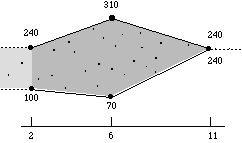
This example describes a uniform random generator for p4 (a frequency ?) and a tendency mask.
The masks range at 2 seconds is {100...240}, therefore the random
numbers are distributed between 100 and 240. The range expands to
{70...310} at 6 seconds and shrinks to a single value of 240 at 11
seconds.
The following forms are special border cases of the mask principle:
1. A mask with a constant lower and a constant upper boundary ist actually a normal (time invariant) range:

Therefore, these two parameter descriptions are equivalent:
p4 rnd uni
mask 10 20
or
p4 range 10 20
2. A mask with constant and identical boundaries describes a constant value:
Therefore, these two parameter descriptions are equivalent:
p4 rnd uni
mask 10 10
or
p4 const 10
3. A mask with time variant but identical boundaries describes a normal segment function - there is no range for random or oscillating numbers:

Therefore, these two parameter descriptions are equivalent:
p4 rnd uni
mask (3 10 5 20 7 10) (3 10 5 20 7 10)
or
p4 seg (3 10 5 20 7 10)
Because of the free choice of an interpolation exponent for segment functions there are a large variety of mask shapes constructed by the same set of break points, for example:
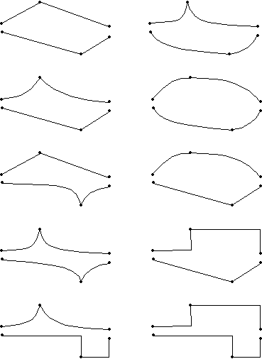
The mathematical transformation (mapping) of the random or periodic values into the mask follows a linear, a power oder a root function.
A linear mapping, probably normal for many CMask applications, expands oder compresses the values to the current mask range in a proportional (linear) way. For example, if the random values 0.0, 0.1, 0.5 and 0.8 will be linear transformed in a range between 2 and 6, the result will be 2.0, 2.4, 4.0 and 5.2. With a range of -10 ... +10 we will have -10.0, -8.0, 0.0, 6.0.
A power function changes the original proportion. A square function transforms the valuea 0.0, 0.1, 0.5 and 0.8 to 0.0, 0.01, 0.25 and 0.64. A mapping into the range [2,6] results in 2.0, 2.04, 3.0 and 4.56.
A square root function, for example, transforms the values to 0.0, 0.316..., 0.707... and 0.894.... In the range [2,6] this is 2.0, 3.264..., 4.828... und 5.577....
The mapping function in CMask is![]()
x is the input value and n the mapping exponent
n=0 gives a linear function.
n>0 gives a power function, n=1 gives the square function.
n<0 gives a root function, n=-1 gives the square root function.
For many synthesis parameters the linear transformation would be the right choice. But if we want to generate uniform distributed frequencies for use in audio oscillators between 100 and 800 Hz for example, they will distributed equally in that range, but we will hear more higher pitches. In this example the half of all frequencies fall in the range 450...800 Hz, this is about 1 octave. The other half (100...450) comprises more than 2 octaves. Therefore pitches from the lowest octave will be rare in relation to the pitches from the highest octave. To solve the problem of the logarithmic frequency-pitch-relation one can either use cent or oct values instead of frequencies or use as approximation an exponential distribution instead of uniform. The third way is a square function as mapping transformation. We have a similar case with onset differences and durations. Uniform distributed time intervals or durations would be perceived as a preference of larger intervals and durations.
After generation and mask mapping it is possible to quantize the numbers. There are 3 parameters for quantization: interval, strength and offset .
The quantization interval is the distance between two neighbouring points in the value range. All these points form an equidistant grid. These points attract surrounding random values like magnets. (Compare with metrical quantize in a MIDI sequencer.)
An interval of 30, for example, builds a grid: .... -120 -90 -60 -30 0 30 60 90 120 150 180 ....
The interval can also be time variant. The segment function
(0 30 5 30 10 45), for
example, describes a grid that is constant before 30 seconds and
increasing after this time:
quant (0 30 5 30 10 45) 1
0

The quantization offset, also controllable by a segment function, is a shift of the grid.
An offset value of 10 and an interval of 30 results in the grid: .... -110 -80 -50 -20 10 40 70 100 130 160 190....
This is an example for a dynamic offset:
quant 40 1 (3 0 6 20)
The quantization strength, a value or a segment function in the range {0...1}, i.e. 0 ... 100%, specify how the grid points attract values between them.
A strength value of 1 gives a total quantization - every random value are now precise on the grid. A strength of 0.5 (50%) means, that all random values are shifted to the half distance to the next grid point. (Compare with "Iterative Quantize" in a sequencer.)
An example for an increasing strength:
quant 40 (0 0 10 1) 0
The example below shows a tendency mask combined with a quantization with dynamic interval, offset and strength (grey areas in the mask are possible areas for random or periodic values):
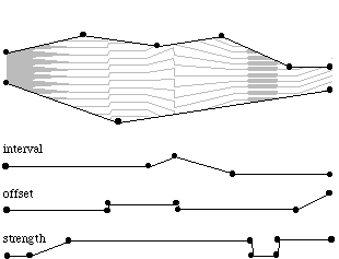
Quantization is useful for the construction of regular meters in rhythm oder harmonic frequency grids.
An accumulator adds all its input values and an initial value together.
For example, the numbers 10 2 34 5 and an inital value of 0 results in 10 12 46 51. That is, one can look upon the input values as relative values or intervals. The numbers after accumulation are absolute values.
If we use an accumulator in connection with a random generator, we can call the result a random walk. Depending on the input values, the sum may rise to a very large number. In order to limit to sum to a certain range it is possible to define lower and upper boundaries similar to a mask. The specification of the accumulation mode prescribes the behavior near to a boundary. The limit - mode cuts values higher than the upper limit and vice versa. The mirror - mode reflects the amount that crosses the limit back into the allowed range. The wrap - mode considers both limits the same, so that a value that is too high comes out above the lower boundary and vice versa.
|
limit |
mirror |
wrap |
|
|
|
|
The lines below describe a field that contains 6 parameter in the valid CMask syntax:
{ f1 0 8193 10 1 ;text in braces take place i3 0 20 ;in the score file unchanged } f 0 10 ;a field from 0 to 10 seconds p1 const 1 ;instrument 1 p2 range .01 .2 prec 3 ;onsets between 10 and 200 ms ;precision: 3 digits after ;the decimal point p3 rnd exp 1 ;durations between 0.5 and 1 seconds mask .5 1 ;and exponential distribution prec 2 p4 item heap (120 125 400 355) ;permutations of 4 values p5 rnd uni ;uniform distributed numbers mask (3 100 8 50) 200 map 1 ;between 100 and 200 at first and ;between 50 and 200 in the end p6 osc cos (0 .5 10 5) ;faster and faster oscillating values;in the range {0...1}
The file format of the parameter file have to be plain ASCII text,
similar to the .orc and .sco files.
Suitable text editors for Csound and CMask on the Mac are
BBedit or
Alpha.
As usual one should design the instruments and the orchestra file
at first. If the meaning of the pfields p4 ... pn is fixed one can write
generators, masks etc. for all the pfields in a parameter file.
If the score file should also contain other note lists or function
table statements one can write these within braces {...} as the first
lines of the parameter file. This part of the parameter file will be
taken unchanged into the score file. In this way one gets a complete
score file for Csound that don't have to be further edited.
Each parameter can have its own precision. The default value for the
decimal places after the point is 5. In order to get integer numbers,
for example, the precision have to be 0.
For a better readability it is advisable to insert comments (after a
semicolon).
CMask on the Macintosh:
After launching CMask a file dialog box appears to select the parameter file. Then one have to set the path and type the name for the new score file. The default for the file name is the name of the parameter file with appended '.sco'. If an errors occurs, CMask stops and prints a message. One have to quit (command-Q) the program now. After debugging one can restart CMask. If the text was OK, CMask writes the score file to the disk.
CMask on SGI:
CMask expects at least on argument: the name of the parameter file. The optional second argument may contain the name for the new score file. If no score file name is given, CMask appends '.sco' to the paramater file name as the new score file name. If an errors occurs, CMask prints a message and stops. After debugging one can restart CMask. If the text was OK, CMask writes the score file to the disk.
CMask on the PC:
There is no GUI for CMask, so you have to run it in a MS-DOS-Window. CMask expects at least on argument: the name of the parameter file. A special file type extension is not required. The optional second argument may contain the name for the new score file. If no score file name is given, CMask appends '.sco' to the paramater file name as the new score file name. If an errors occurs, CMask prints a message and stops. After debugging one can restart CMask. If the text was OK, CMask writes the score file to the disk.